Use of the timevar() option
Background
In this tutorial I will describe some simple use of the timevar() option when obtaining predictions after fitting a model using stpm2. When using Stata’s survival models, such as streg and stcox, predictions are made at the values of _t, which is each record’s event or censoring time. This is the default behaviour of stpm2.
One of the advantages of parametric survival models is that we can predict various quantities (hazard, survival functions etc etc) at any value of time and for any covariate pattern as we have an equation which is a function of time and any covariates we have modelled.
Before I show some examples I should explain that we need to be a bit cautious when making such predictions. In Stata it is only possible to have one data set in memory. When we make predictions at specific values of time using the timevar() option we effectively want a second data set that we can use for predictions, and then use for producing graphs and tabulations.
We have found it easiest to think of two data sets side by side as shown below.
------------------  --------------
|                |  |            |
|                |  | Prediction |
| Analysis Data  |  |    Data    |
|                |  |            |
|                |  --------------
|                |
------------------
This means that we have our analysis data and our prediction data stored in the same data set. We have to remember that there are actually two (or more) data sets and that row 1 or the analysis data does not have a relationship with row 1 of the prediction data.
I now will illustrate the use of the timevar() option.
Example
I first load and stset the rott2b data.
. use https://www.pclambert.net/data/rott2b, clear
(Rotterdam breast cancer data (augmented with cause of death))

. stset rf, f(rfi==1) scale(12) exit(time 60)

     failure event:  rfi == 1
obs. time interval:  (0, rf]
 exit on or before:  time 60
    t for analysis:  time/12

------------------------------------------------------------------------------
      2,982  total observations
          0  exclusions
------------------------------------------------------------------------------
      2,982  observations remaining, representing
      1,181  failures in single-record/single-failure data
 11,130.825  total analysis time at risk and under observation
                                                at risk from t =         0
                                     earliest observed entry t =         0
                                          last observed exit t =         5
I will model the effect of age using restricted cubic splines. These can be generated using the rcsgen command. I make use of the center option make the created spline variables all equal 0 at the specified value, in this case at age 60. I then fit an stpm2 model including the effect of hormonal therapy (hormon), progesterone receptor (transformed using
. rcsgen age, df(3) gen(agercs) center(60)
Variables agercs1 to agercs3 were created

. stpm2 hormon agercs* pr_1, scale(hazard) df(4) eform

Iteration 0:   log likelihood = -3065.3989
Iteration 1:   log likelihood = -3065.2479
Iteration 2:   log likelihood = -3065.2478

Log likelihood = -3065.2478                     Number of obs     =      2,982

------------------------------------------------------------------------------
             |     exp(b)   Std. Err.      z    P>|z|     [95% Conf. Interval]
-------------+----------------------------------------------------------------
xb           |
      hormon |   1.253481    .112407     2.52   0.012     1.051442    1.494342
     agercs1 |   .9678468   .0119668    -2.64   0.008     .9446742    .9915879
     agercs2 |    .999971   .0000315    -0.92   0.357     .9999092    1.000033
     agercs3 |   1.000014   .0000304     0.46   0.648     .9999543    1.000074
        pr_1 |   .9080251   .0118154    -7.41   0.000     .8851601    .9314808
       _rcs1 |   2.464395   .0655981    33.88   0.000     2.339121    2.596377
       _rcs2 |   1.227705   .0289332     8.70   0.000     1.172287    1.285744
       _rcs3 |   1.013422   .0117182     1.15   0.249     .9907135    1.036652
       _rcs4 |   1.005574   .0050256     1.11   0.266      .995772    1.015472
       _cons |   .3891571   .0248262   -14.79   0.000     .3434176    .4409885
------------------------------------------------------------------------------
Note: Estimates are transformed only in the first equation.
I now create some values of time that I want to predict at. I use the range command to give 100 values between 0 and 5 in a new variable tt.
. range tt 0 5 100
(2,882 missing values generated)
After creating the new variable I can use it in the timevar() option when using stpm2’s predict command.
. predict s0, survival timevar(tt) zeros ciThis will predict the baseline survival function at the time values in the variable tt. The zeros option sets all covarites equal to zero, i.e. the baseline. The ci option asks for the upper and lower bounds of the 95% confidence interval to be calculated. The function can now be plotted.
. twoway (rarea s0_lci s0_uci tt, color(blue%25)) ///
>                 (line s0 tt, lcolor(red)) ///
>                 , legend(off) ///
>                 ylabel(,angle(h) format(%3.1f)) ///
>                 xtitle("Years from surgery") ///
>                 ytitle("S(t)")
Combining with the at() option.
It is possible to make predictions at any values the covariates included in the model using the at() option. The two lines below predict the hazard functions for women using and not using hormonal treatment at the reference age (60) and the mean value of log progesterone receptor (3.43).
. predict h0, hazard timevar(tt) at(hormon 0 pr_1 3.43) zeros per(1000) ci

. predict h1, hazard timevar(tt) at(hormon 1 pr_1 3.43) zeros per(1000) ci
I have used the timevar(tt) option again and so predictions will be at the 100 value of tt (actually at 99 values as the hazard is not defined at t=0). The at() option gives the values of the covariates that we want to predict at. The zeros option will set any remaining covariates equal to zero, i.e. the age spline variables are set to zero which is the reference age of 60. The per(1000) option multiplies the hazard rate by 1000 as it is easier to interpret the rate per 1000 years than per person per year.
The resulting predictions are then plotted,
. twoway  (rarea h0_lci h0_uci tt, color(red%25)) ///
>                 (rarea h1_lci h1_uci tt, color(blue%25)) ///
>                 (line h0 tt, lcolor(red) lwidth(thick)) ///
>                 (line h1 tt, lcolor(blue) lwidth(thick)) ///
>                 ,xtitle("Years from surgery") ///
>                 ytitle("Recrurrence rate (per 1000 py)") ///
>                 legend(order( 3 "hormon=0" 4 "hormon=1") ring(0) pos(1) cols(1))
As the model assumes proportional hazards the predicted hazard functions are perfectly proportional.
Predictions at single values of time.
It can be useful to see the variation in survival at specific values of time, for example at one and five years. The followig code predicts the survival at one year for all subjects in the dataset.
. gen t1 = 1

. predict s_time1, survival timevar(t1)
This can then be plotted in a histogram.
. hist s_time1, width(0.02) xlab(0.3(0.1)1) name(t1, replace)
(bin=7, start=.81623113, width=.02)
We can compare this to the variation at 5 years.
. gen t5 = 5

. predict s_time5, survival timevar(t5)

. hist s_time5, width(0.02) xlab(0.3(0.1)1)  name(t5, replace)
(bin=22, start=.30392122, width=.02)
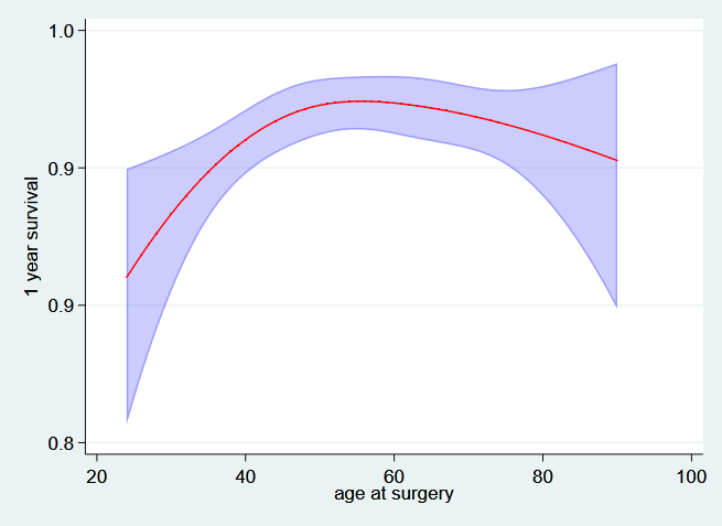
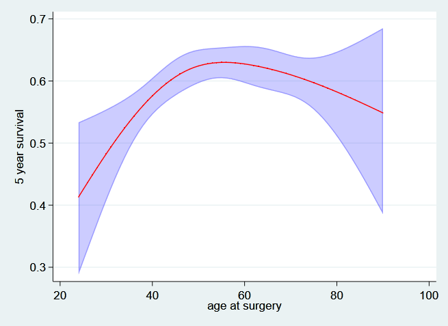
If we are interested in specific covariates then we can look at 1 and 5 year survival as a function of that covariate. For example, we can plot the 1 and 5 year survival as a function of age at diagnosis. As this will also depend on the values of the other covariate I will fix these at specific values (not on hormonal treatment and at the mean level of log progesterone receptor).
First the one year survival as a function of age,
. predict t1_age, surv at(hormon 0 pr_1 3.43) ci timevar(t1)

. twoway  (rarea t1_age_lci t1_age_uci age, sort color(blue%25))  ///
>                 (line t1_age age, sort lcolor(red)) ///
>                 ,ytitle("1 year survival") legend(off) ///
>                 ylabel(,angle(h) format(%3.1f)) name(age_t1, replace)
And now the 5 year survival….
. predict t5_age, surv at(hormon 0 pr_1 3.43) ci timevar(t5)

. twoway  (rarea t5_age_lci t5_age_uci age, sort color(blue%25))  ///
>                 (line t5_age age, sort lcolor(red)) ///
>                 ,ytitle("5 year survival") legend(off) ///
>                 ylabel(,angle(h) format(%3.1f)) name(age_t5, replace)